

CDNOW: from a raw transaction log to lifetime value#
Audience. An analyst who believes CLV is average ticket x frequency x margin, is comfortable with pandas, and has never met the buy-till-you-die literature.
Prerequisites. uv sync in the repo root. No network and no API keys. The CDNOW sample ships with the repository.
Learning goals. By the end you can:
Define frequency, recency and T the way this literature defines them, which is not the way RFM defines two of them.
Turn a raw transaction log into a
CustomerBase, and say whytime_unitandcollapseare two arguments rather than one.Reproduce the published Fader, Hardie & Lee (2005) BG/NBD estimates on CDNOW, then check the fit against 39 weeks it never saw.
Compose a transaction model and a spend model into discounted lifetime value, and get the numbers back out as a DataFrame.
Nothing below assumes you’ve read a BTYD paper. Section 0 builds the vocabulary from scratch, and every term it defines gets drawn on real customers in section 2.
Outline#
The vocabulary, and the word that trips everyone
Load the raw log
Four customers, drawn
CustomerBase, and its two questions about timeReproducing the published estimates
What happens if you get recency wrong
Predicted against actual, on the holdout
Lifetime value, plotted and exported
What
time_unit="W"does on its ownExercise
0. The vocabulary, and the word that trips everyone#
What the models are actually looking at#
Every model in clvkit reads one thing: a transaction log. That’s a table with one row per purchase, carrying who bought, when, and optionally how much.
customer_id        date   amount
          1  1997-01-01    11.77
          1  1997-01-18    89.00
          2  1997-01-01    45.55
That’s all. No demographics, no channel, no campaign. The claim these models make is that the timing of somebody’s past purchases predicts their future ones, and they’d rather be judged on that than on features they can’t get.
From the log, clvkit computes four numbers per customer. Those four numbers are the whole interface between your data and the maths.
The glossary#
Term |
What it means here |
Watch out |
|---|---|---|
Transaction log |
One row per purchase: who, when, how much. |
Not one row per SKU. A basket is one purchase. |
Purchase event |
One shopping trip, after same-period purchases are merged. |
Two orders on the same day are one event. |
``frequency`` |
The number of repeat purchases. Total purchases minus one. |
A customer who bought 3 times has |
``recency`` ( |
Time from the customer’s first purchase to their last one. |
This is not “time since the last purchase”. See below. |
``T`` |
The customer’s age: time from their first purchase to the end of the observation window. |
Per customer, not a calendar constant. Two customers observed on the same day have different |
``monetary_value`` |
Average amount per repeat purchase. |
The first purchase is excluded, which surprises people. |
BTYD |
“Buy till you die”, the family of models here. |
A name nobody outside the field uses. |
``P(alive)`` |
Probability the customer hasn’t silently churned by the end of the window. |
Nobody cancels anything in this world, so churn is never observed. It’s inferred from silence. |
Calibration / holdout |
Fit on the first slice of time, test on the rest. |
The holdout is behaviour the fit never saw. |
CLV |
Discounted expected revenue (or margin) over a future horizon. |
Residual value, from now forward. It doesn’t include what the customer already spent. |
The word that trips everyone: recency#
Ask anyone what recency means and you’ll get: today minus the last purchase. A customer who bought 10 days ago has a recency of 10. That’s the RFM definition, it’s a perfectly good definition, and it isn’t the one used here.
In BTYD, recency is t_x: the time from the customer’s first purchase to their last one. The two definitions point at opposite ends of the same timeline, which is easier to see drawn than described.
[1]:
import matplotlib.pyplot as plt

# Chart colours fixed by role and reused across this notebook, validated as a set
# for colour-vision deficiency. Every span also carries a direct label, so nothing
# here depends on telling two hues apart.
SURFACE, INK, MUTED, GUIDE = "#fcfcfb", "#0b0b0b", "#52514e", "#c9c8c3"
ACTIVE, SILENCE, PURCHASE = "#2a78d6", "#eb6834", "#1baf7a"

T, T_X = 100, 62  # one imaginary customer: age 100, last purchase at 62

fig, ax = plt.subplots(figsize=(10.5, 3.5))
fig.patch.set_facecolor(SURFACE)
ax.set_facecolor(SURFACE)

# The three moments, with a dashed guide dropping through every band.
for x, label in [(0, "first purchase"), (T_X, "last purchase"), (T, "end of window")]:
    ax.plot([x, x], [0.15, 3.05], color=GUIDE, lw=1, ls=(0, (3, 3)), zorder=1)
    ax.text(x, 3.2, label, ha="center", fontsize=10, color=INK)

# The customer's own timeline, with purchases on it.
ax.plot([0, T], [2.75, 2.75], color=GUIDE, lw=2, zorder=2)
ax.scatter(
    [0, 18, 40, T_X],
    [2.75] * 4,
    s=95,
    color=PURCHASE,
    edgecolor=SURFACE,
    linewidth=1.6,
    zorder=3,
)
ax.text(T + 3, 2.75, "purchases", va="center", fontsize=9.5, color=PURCHASE)


def span(y, x0, x1, colour, title, subtitle):
    ax.annotate(
        "",
        xy=(x0, y),
        xytext=(x1, y),
        arrowprops={"arrowstyle": "<->", "color": colour, "lw": 2},
    )
    ax.text((x0 + x1) / 2, y + 0.20, title, ha="center", fontsize=11, color=colour)
    ax.text((x0 + x1) / 2, y - 0.34, subtitle, ha="center", fontsize=9, color=MUTED)


span(1.95, 0, T_X, ACTIVE, "recency  (t_x)", "what clvkit calls recency")
span(1.95, T_X, T, SILENCE, "the silence", "what RFM calls recency:  T - t_x")
span(0.80, 0, T, INK, "T  (age)", "first purchase to the end of the window")

ax.set_xlim(-16, 128)
ax.set_ylim(0.30, 3.5)
ax.axis("off")
fig.tight_layout()
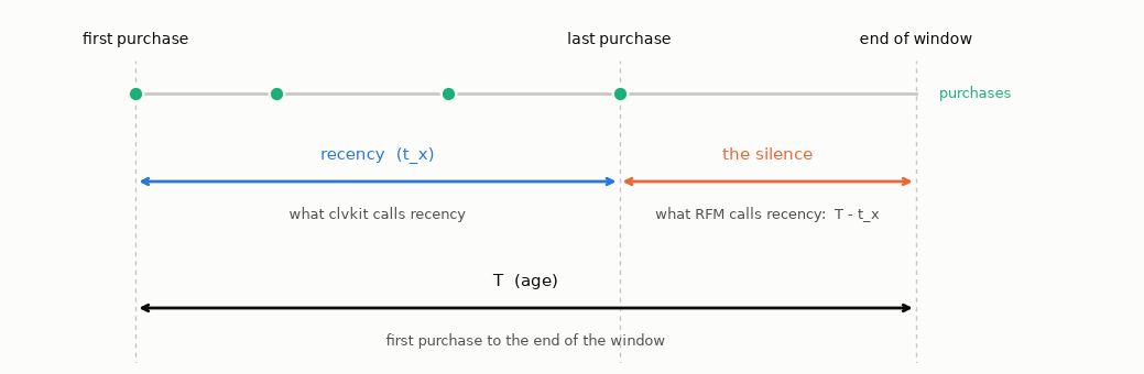
So the two are one subtraction apart, and neither is more correct than the other. But the name collides, and a table built with one definition and read with the other is silently inverted.
Why the papers chose this end#
The BG/NBD likelihood is written over the triple (x, t_x, T). To judge whether somebody has quietly stopped buying, the model needs two spans and not one:
how long the customer was demonstrably active, from 0 to
t_xhow long the whole window lasted, from 0 to
T
The trailing silence, T - t_x, is what drives P(alive) down. But six months of silence means something different for a customer who was active for two years than for one who bought twice in a fortnight and left. Only keeping both spans lets the model tell those apart. Store “days since last purchase” alone and you’ve thrown the comparison away.
You’ll never have to compute any of this yourself. CustomerBase.from_transactions takes the raw log and does it. The reason to know it anyway is that the moment you hand-build a summary table and feed it in, this is the mistake you’ll make, and section 5 shows what it costs.
1. Load the raw log#
CDNOW_sample.txt is the 1/10 systematic sample of the CDNOW cohort. 2,357 customers made their first purchase in the first quarter of 1997 and were tracked through June 1998. Every published Fader-Hardie estimate was fit on this sample rather than on the 23,570-customer master file, so the sample is what a reproduction has to use.
The file is whitespace-separated with no header. Its five columns are the master-file id, the sample id, the date as YYYYMMDD, the number of CDs, and the dollar value.
[2]:
from pathlib import Path

import pandas as pd

from clvkit import BGNBD, CLV, CustomerBase

# Resolved by walking up, so the notebook runs from the repo root or from
# examples/. Outputs are anchored to examples/output/, which .gitignore covers;
# Path.cwd() would scatter them wherever the kernel happened to start.
REPO = next(
    p for p in [Path.cwd(), *Path.cwd().parents] if (p / "CDNOW_sample.txt").exists()
)
OUTPUT = REPO / "examples" / "output"
OUTPUT.mkdir(parents=True, exist_ok=True)

log = pd.read_csv(
    REPO / "CDNOW_sample.txt",
    sep=r"\s+",
    header=None,
    names=["master_id", "customer_id", "date", "quantity", "amount"],
)
log["date"] = pd.to_datetime(log["date"], format="%Y%m%d")

print(f"{len(log):,} transactions, {log['customer_id'].nunique():,} customers")
log.head()
6,919 transactions, 2,357 customers
[2]:
| master_id | customer_id | date | quantity | amount | |
|---|---|---|---|---|---|
| 0 | 4 | 1 | 1997-01-01 | 2 | 29.33 |
| 1 | 4 | 1 | 1997-01-18 | 2 | 29.73 |
| 2 | 4 | 1 | 1997-08-02 | 1 | 14.96 |
| 3 | 4 | 1 | 1997-12-12 | 2 | 26.48 |
| 4 | 21 | 2 | 1997-01-01 | 3 | 63.34 |
2. Four customers, drawn#
Definitions are easier to trust once you’ve seen them measured. These four are real rows of the file, picked because they tell four different stories.
Everything in the next cell is plain pandas on the raw log. No clvkit yet. The point is that frequency, recency and T are arithmetic on dates, and you could do it by hand if you had to.
[3]:
# Same three roles as the schematic in section 0: active span, silence, purchase.
# Ordered most-alive to least, so the diagram reads as a gradient down the page.
CASES = {
    1: "a regular",
    1673: "arrived in March, still buying at the end",
    18: "two purchases, then 17 months of silence",
    4: "bought once, never came back",
}

end_of_window = log["date"].max()
trips = (
    log.assign(day=log["date"].dt.normalize())
    .drop_duplicates(["customer_id", "day"])  # same-day orders are one trip
    .groupby("customer_id")["day"]
)

rows = []
for cid in CASES:
    days = trips.get_group(cid).sort_values()
    first = days.min()
    rows.append(
        {
            "customer_id": cid,
            "offsets": (days - first).dt.days.to_numpy(),
            "frequency": len(days) - 1,  # REPEAT purchases: total minus one
            "recency": (days.max() - first).days,  # first -> last
            "T": (end_of_window - first).days,  # first -> end of window
        }
    )
by_hand = pd.DataFrame(rows).set_index("customer_id")
by_hand[["frequency", "recency", "T"]]
[3]:
| frequency | recency | T | |
|---|---|---|---|
| customer_id | |||
| 1 | 3 | 345 | 545 |
| 1673 | 2 | 457 | 485 |
| 18 | 1 | 34 | 545 |
| 4 | 0 | 0 | 545 |
[4]:
fig, ax = plt.subplots(figsize=(11, 4.4))
fig.patch.set_facecolor(SURFACE)
ax.set_facecolor(SURFACE)

for row, (cid, note) in enumerate(CASES.items()):
    y = len(CASES) - row - 1
    r = by_hand.loc[cid]

    # The active span, then the silence. Two spans, one row, no overlap.
    ax.plot([0, r["recency"]], [y, y], color=ACTIVE, lw=9, solid_capstyle="butt")
    ax.plot([r["recency"], r["T"]], [y, y], color=SILENCE, lw=9, solid_capstyle="butt")
    ax.scatter(
        r["offsets"],
        [y] * len(r["offsets"]),
        s=70,
        color=PURCHASE,
        edgecolor=SURFACE,
        linewidth=1.5,
        zorder=3,
    )

    # Notes start at a fixed x so their left edges line up into a column.
    ax.text(575, y, note, va="center", fontsize=9, color=MUTED)
    ax.text(-14, y + 0.10, f"#{cid}", va="center", ha="right", fontsize=10, color=INK)
    ax.text(
        -14,
        y - 0.20,
        f"x={r['frequency']}  t_x={r['recency']}  T={r['T']}",
        va="center",
        ha="right",
        fontsize=8,
        color=MUTED,
    )

# The spans are labelled on the chart, not left to a colour key. Both labels sit
# over customer 1, the only row long enough to show the two spans at full length.
top = len(CASES) - 1
ax.text(
    172,
    top + 0.30,
    "recency (t_x): first purchase to last",
    fontsize=9,
    color=ACTIVE,
    ha="center",
)
ax.text(445, top + 0.30, "the silence: T - t_x", fontsize=9, color=SILENCE, ha="center")
ax.annotate(
    "a purchase event",
    xy=(0, 0),
    xytext=(140, -0.66),
    fontsize=9,
    color=PURCHASE,
    ha="center",
    arrowprops={"arrowstyle": "-", "color": PURCHASE, "lw": 1},
)

ax.set_xlim(-210, 770)
ax.set_ylim(-0.95, len(CASES) - 0.30)
ax.set_yticks([])
ax.set_xticks(range(0, 601, 100))
ax.set_xlabel("Days since that customer's own first purchase", color=MUTED)
ax.set_title("frequency, recency and T, measured on four CDNOW customers", loc="left")
for side in ("top", "right", "left"):
    ax.spines[side].set_visible(False)
ax.spines["bottom"].set_color("#d8d7d2")
ax.tick_params(colors=MUTED)
fig.tight_layout()
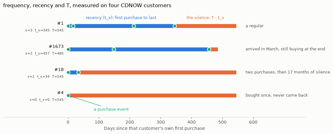
Four things that diagram is trying to make obvious.
Customer 4 has ``frequency = 0`` and did buy something. Frequency counts repeat purchases, so a one-time buyer is a 0. His recency is 0 too, because his first and last purchase are the same event, and the blue span has no length at all.
Customer 18 has ``recency = 34`` and hasn’t bought in 511 days. Under the RFM definition his recency would be 511. Same customer, same file, two numbers that differ by a factor of 15.
Customer 1673 has ``T = 485`` while the others have 545. He arrived on 2 March 1997, two months after the rest, so his window is shorter. T is measured from each customer’s own first purchase, which is why it isn’t a property of the calendar.
The orange span is the part the model is suspicious about. Long orange after a short blue reads as churn. Long orange after a long blue reads as a lapse. Customer 1673 has almost no orange, and he’s the one the model will treat as most alive.
3. CustomerBase, and its two questions about time#
CustomerBase.from_transactions is the single seam every clvkit model consumes. It takes two separate time arguments, and collapsing them into one is the expensive mistake available here.
time_unit is the ruler. It is the unit recency and T get reported in. collapse is the event grain. Transactions falling in the same period become one purchase, because the counting process these models assume wants separated events.
The published CDNOW fit answers the two questions differently. Purchases collapse at the data’s own daily resolution, since CDNOW records a date and two orders on one date are one shopping trip. Time itself is measured continuously in weeks: for customer i, “T_i = 39 - time of first purchase”. That is time_unit="W", collapse="D".
amount_col=None here because BG/NBD only looks at timing. It also keeps all 2,357 customers, since netting negative amounts would drop the eight whose only calibration transaction has a zero dollar value.
Start at daily grain, so the output is directly comparable to the arithmetic done by hand in section 2.
[5]:
cb_days = CustomerBase.from_transactions(
    log, amount_col=None, time_unit="D", collapse="D"
)
check = cb_days.to_pandas().loc[list(CASES)]
print(check)
print()
print(
    "matches the by-hand table:", check.equals(by_hand[["frequency", "recency", "T"]])
)
             frequency  recency    T
customer_id
1                    3      345  545
1673                 2      457  485
18                   1       34  545
4                    0        0  545

matches the by-hand table: True
Same four numbers. from_transactions isn’t doing anything mysterious, it’s doing the date arithmetic from section 2 for all 2,357 customers at once and keeping a record of the choices it made.
Now the ruler changes. The published CDNOW fit is reported in weeks, so T = 545 days becomes T = 77.86 weeks.
[6]:
cb_timing = CustomerBase.from_transactions(
    log, amount_col=None, time_unit="W", collapse="D"
)
print(cb_timing)
CustomerBase  2,357 customers, 1,139 repeat (48%)
-------------------------------------------------------------------------------------------------------
        ruler  time_unit='W'    -> recency and T are counted in 'W'
        grain  collapse='D'     -> events kept at 'D', reported in 'W'
      amounts  no               -> built with amount_col=None
    negatives  'net'            -> netted per period; periods not staying positive were dropped
  observed to  1998-06-30       -> 78 W of history at the oldest customer

         fits  BGNBD  MBGNBD  CohortSurvival
      refused  GammaGamma, CLV  -> no spend column to model

         note  52% bought once - the models see them only through the population, not their own history
print(cb) is the long form and repr(cb) is the one line you get inside a list or a traceback. Read the ruler and grain rows above: they’re the record of the two answers, and they’re what stops a base built one way from being read as if it were built another.
The note line at the bottom is worth pausing on. 52% of this base bought exactly once, so for half these customers the model has frequency = 0 and recency = 0, and it can only describe them through the population. That’s not a defect of the data, it’s what a retail base looks like, and it’s the reason these models are built on a population prior rather than on per-customer curve fitting.
[7]:
cb_timing.to_pandas().head()
[7]:
| frequency | recency | T | |
|---|---|---|---|
| customer_id | |||
| 1 | 3 | 49.285714 | 77.857143 |
| 2 | 1 | 1.714286 | 77.857143 |
| 3 | 0 | 0.000000 | 77.857143 |
| 4 | 0 | 0.000000 | 77.857143 |
| 5 | 0 | 0.000000 | 77.857143 |
4. Reproducing the published estimates#
Fader, Hardie & Lee (2005) §7 calibrate the BG/NBD on the first 39 of the 78 weeks and report r = .243, alpha = 4.414, a = .793, b = 2.426. The Excel worksheet screenshot in their Figure 1 shows exactly those four cells, alongside a maximised log-likelihood of -9582.4.
split() recomputes calibration RFM against a cut date exactly as from_transactions would, and hands back the holdout behaviour alongside it.
[8]:
calibration, holdout = cb_timing.split(calibration_period_end="1997-09-30")
model = BGNBD().fit(calibration)

published = pd.Series(
    {"r": 0.243, "alpha": 4.414, "a": 0.793, "b": 2.426}, name="published"
)
comparison = pd.DataFrame({"fitted": model.params_, "published": published})
comparison["abs_error"] = (comparison["fitted"] - comparison["published"]).abs()

print(f"customers in calibration: {len(calibration.to_pandas()):,}")
print(f"log-likelihood: {model.log_likelihood_:.1f}  (published -9582.4)")
comparison
customers in calibration: 2,357
log-likelihood: -9582.4  (published -9582.4)
[8]:
| fitted | published | abs_error | |
|---|---|---|---|
| r | 0.242595 | 0.243 | 0.000405 |
| alpha | 4.413602 | 4.414 | 0.000398 |
| a | 0.792922 | 0.793 | 0.000078 |
| b | 2.425907 | 2.426 | 0.000093 |
Alpha comes out 4.413602 against a published 4.414. Every parameter agrees to within half a unit in the last digit the paper prints, which is the strongest claim available against a three-decimal published table. The repository’s golden test asserts the same thing on every CI run, so the numbers above can’t quietly drift.
How sure are those four numbers?#
Four point estimates and no error bars. parameter_uncertainty puts intervals on them with a parametric bootstrap: simulate 100 synthetic customer bases from the fitted parameters, refit the model on each, and read the spread of the refits. Nothing here runs unless you call it, and the price is what it sounds like, 100 refits, about half a minute on this base.
[9]:
uncertainty = model.parameter_uncertainty(n=100, seed=42)
uncertainty.plot()
uncertainty.to_pandas().round(3)
[9]:
| estimate | se | ci_low | ci_high | |
|---|---|---|---|---|
| parameter | ||||
| r | 0.243 | 0.012 | 0.219 | 0.269 |
| alpha | 4.414 | 0.359 | 3.755 | 5.237 |
| a | 0.793 | 0.176 | 0.518 | 1.184 |
| b | 2.426 | 0.636 | 1.532 | 3.934 |
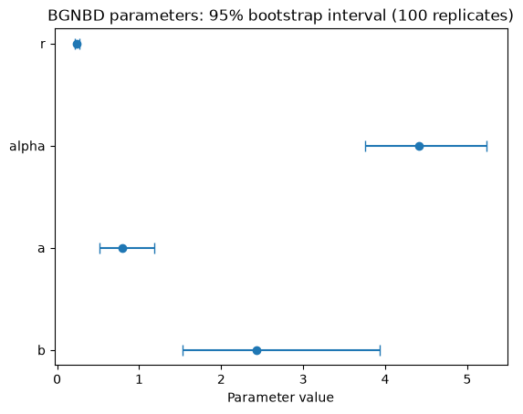
r is pinned: 0.243 sits inside [0.219, 0.269]. The dropout pair isn’t. a spans [0.518, 1.184] and b spans [1.532, 3.934], intervals nearly as wide as the estimates themselves. So the same 2,357 customers that reproduce a published table to three decimals only weakly identify where dropout risk sits, and both facts are true at once. The exercise in section 9 swaps in MBGNBD, which answers with the same result type from its own parameter_uncertainty.
There’s now a fitted model in hand, which means section 0’s warning about recency can stop being a warning and become a measurement.
5. What happens if you get recency wrong#
Suppose you skip from_transactions, build the summary table yourself in SQL, and fill recency with the RFM definition: days since the last purchase. Every column name is right. Every value is a plausible non-negative number. Nothing raises.
Below, the same fitted model scores the same customers twice. Once with t_x, and once with the summary table’s recency column replaced by T - t_x.
[10]:
correct = cb_days.to_pandas()

# The same table, with recency filled the RFM way: time since the last purchase.
rfm_style = correct.copy()
rfm_style["recency"] = rfm_style["T"] - rfm_style["recency"]

cb_rfm = CustomerBase(
    rfm_style,
    time_unit="D",
    observation_period_end=cb_days.observation_period_end,
    has_monetary=False,
    on_negative="net",
)

model_days = BGNBD().fit(cb_days)
side_by_side = correct.copy()
side_by_side["P_alive"] = model_days.probability_alive().to_pandas()
side_by_side["P_alive_rfm_recency"] = model_days.probability_alive(cb_rfm).to_pandas()

side_by_side.loc[list(CASES)].round(3)
[10]:
| frequency | recency | T | P_alive | P_alive_rfm_recency | |
|---|---|---|---|---|---|
| customer_id | |||||
| 1 | 3 | 345 | 545 | 0.661 | 0.293 |
| 1673 | 2 | 457 | 485 | 0.841 | 0.054 |
| 18 | 1 | 34 | 545 | 0.241 | 0.802 |
| 4 | 0 | 0 | 545 | 1.000 | 1.000 |
[11]:
fig, ax = plt.subplots(figsize=(9, 3.6))
fig.patch.set_facecolor(SURFACE)
ax.set_facecolor(SURFACE)

shown = side_by_side.loc[list(CASES)]
y = range(len(shown))
height = 0.36

ax.barh(
    [i + height / 2 for i in y],
    shown["P_alive"],
    height=height,
    color=ACTIVE,
    label="recency = t_x (correct)",
)
ax.barh(
    [i - height / 2 for i in y],
    shown["P_alive_rfm_recency"],
    height=height,
    color=SILENCE,
    label="recency = days since last purchase",
)

for i, (_, r) in enumerate(shown.iterrows()):
    ax.text(
        r["P_alive"] + 0.015,
        i + height / 2,
        f"{r['P_alive']:.2f}",
        va="center",
        fontsize=9,
        color=MUTED,
    )
    ax.text(
        r["P_alive_rfm_recency"] + 0.015,
        i - height / 2,
        f"{r['P_alive_rfm_recency']:.2f}",
        va="center",
        fontsize=9,
        color=MUTED,
    )

ax.set_yticks(list(y), [f"#{cid}\n{CASES[cid]}" for cid in shown.index], fontsize=8)
ax.invert_yaxis()  # same top-to-bottom order as the timeline above
ax.set_xlim(0, 1.12)
ax.set_xlabel("P(alive) at the end of the window", color=MUTED)
ax.set_title("The same model, the same customers, one column swapped", loc="left")
# Below the axes, because the bars reach 1.0 and leave no room inside the plot.
ax.legend(
    loc="upper center", bbox_to_anchor=(0.5, -0.26), ncol=2, frameon=False, fontsize=9
)
for side in ("top", "right", "left"):
    ax.spines[side].set_visible(False)
ax.spines["bottom"].set_color("#d8d7d2")
ax.tick_params(colors=MUTED)
fig.tight_layout()
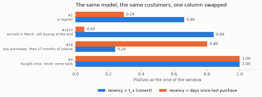
Customer 1673 is the one to look at. He bought three times, the last of them 28 days before the window closed, and he’s the most obviously alive customer on the page. With t_x the model puts him at 0.84. With RFM recency in the column he drops to 0.05.
Customer 18 goes the other way. He last bought on 4 February 1997 and never returned across the following 511 days. Correct scoring gives him 0.24. The broken column reads “last seen on day 511 of 545” and lifts him to 0.80.
So the failure isn’t noise, it’s an inversion. It promotes the dead and demotes the living, which is the single thing this model exists to avoid. Customer 4 is the cruel detail: he scores 1.00 either way, because his recency and his T - recency are both consistent with a one-time buyer, so any spot-check that happens to land on a one-time buyer confirms the code is fine.
And nothing surfaces it. No exception, no warning, a P(alive) column full of numbers between 0 and 1, and a win-back campaign aimed at exactly the wrong list.
The defence is to not build the table. CustomerBase.from_transactions reads the raw log, so there’s no column left for you to fill in with the wrong definition.
6. Predicted against actual, on the holdout#
Parameters can print correctly while the forecast is wired wrong, so matching the published numbers isn’t the last word. The stronger check: bucket customers by how many repeat purchases they made during calibration, then compare mean predicted holdout purchases against mean actual, bucket by bucket, over 39 weeks the fit never saw. The sparse right tail collapses into a “7+” bucket.
[12]:
HOLDOUT_WEEKS = 39

forecast = model.predict(t=HOLDOUT_WEEKS).to_pandas()
joined = (
    calibration.to_pandas()
    .join(forecast)
    .join(holdout["frequency_holdout"])
    .assign(bucket=lambda d: d["frequency"].clip(upper=7))
)

by_bucket = joined.groupby("bucket").agg(
    customers=("frequency", "size"),
    predicted=("expected_purchases", "mean"),
    actual=("frequency_holdout", "mean"),
)
by_bucket.round(3)
[12]:
| customers | predicted | actual | |
|---|---|---|---|
| bucket | |||
| 0 | 1411 | 0.225 | 0.237 |
| 1 | 439 | 0.523 | 0.697 |
| 2 | 214 | 1.044 | 1.393 |
| 3 | 100 | 1.520 | 1.560 |
| 4 | 62 | 2.164 | 2.532 |
| 5 | 38 | 2.654 | 2.947 |
| 6 | 29 | 3.504 | 3.862 |
| 7 | 64 | 6.157 | 6.359 |
[13]:
fig, ax = plt.subplots(figsize=(7, 4))
ax.plot(by_bucket.index, by_bucket["actual"], marker="o", label="actual")
ax.plot(by_bucket.index, by_bucket["predicted"], marker="s", label="predicted")
ax.set_xlabel("Calibration repeat purchases (7+ collapsed)")
ax.set_ylabel(f"Mean purchases in weeks 40-{39 + HOLDOUT_WEEKS}")
ax.set_title("Conditional expectation against holdout behaviour")
ax.legend()
fig.tight_layout()
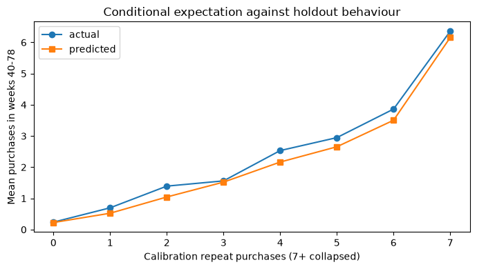
The two lines stay within half a purchase of each other in every bucket, and the worst cell is bucket 4 at 0.368.
Look at the direction, though. The model predicts low in every bucket except 0. Bucket 1 forecasts 0.523 against an actual 0.697, which is 25% short. That is a systematic downward bias, not scatter, and it’s the number worth carrying away from this section: the fit is good enough to publish and still leaves money on the table for the customers who came back once.
What’s being claimed here isn’t that the optimiser converged. It’s that the optimiser converged onto behaviour the model was never shown.
7. Lifetime value, plotted and exported#
Lifetime value is a monetary quantity, so it needs a base built with amounts. CLV is one multiplication:
CLV = margin x revenue per purchase x DET
DET is the number of discounted expected transactions, which is the “how often” half. Revenue per purchase is the “how much” half. CLV defaults to BGNBD() for the first and GammaGamma() for the second, and takes either as an argument to swap it.
discount_rate is the rate per time_unit, not per year. At weekly granularity 0.001 is 0.1% a week, roughly 5% a year. Getting that wrong by a factor of 52 is easy and the number still looks plausible, which is why the argument is documented in the unit the base is in.
[14]:
cb = CustomerBase.from_transactions(log, time_unit="W", collapse="D")
clv = CLV().fit(cb)
print(repr(clv))

result = clv.predict(horizon=12, discount_rate=0.001, margin=1.0)
print(repr(result))
result.to_pandas().head()
<CLV BGNBD x GammaGamma (fitted on W)>
<CLVResult horizon=12 W, discount_rate=0.001, margin=1, 2349 customers>
[14]:
| expected_purchases | discounted_expected_transactions | expected_spend | clv | |
|---|---|---|---|---|
| customer_id | ||||
| 1 | 0.301136 | 0.299205 | 25.960034 | 7.767369 |
| 2 | 0.029539 | 0.029349 | 21.510459 | 0.631317 |
| 3 | 0.036133 | 0.035901 | 35.812712 | 1.285705 |
| 4 | 0.036133 | 0.035901 | 35.812712 | 1.285705 |
| 5 | 0.036133 | 0.035901 | 35.812712 | 1.285705 |
How to read a row#
Four columns, and the last one is the first three multiplied. Take customer 1.
Column |
Value |
What it is |
|---|---|---|
|
1.202 |
Purchases expected over the next 52 weeks |
|
1.172 |
The same purchases, brought back to today’s money |
|
25.96 |
What he spends per purchase |
|
30.42 |
|
1.2 purchases is an average, not a forecast. Nobody buys 1.2 times. It’s the whole distribution collapsed to its mean, and most of that mean is the model hedging on whether he’s still a customer at all. The next cell shows the hedge.
The discount costs 2.5%. 1.202 becomes 1.172 because discount_rate=0.001 is 0.1% a week and the purchases land spread across the year. Pass discount_rate=0 and the two columns come out identical.
``expected_spend`` is not his own average. He spent 23.72 per repeat purchase. The model says 25.96, pulled toward what the population does. Three repeat purchases isn’t much evidence, so it doesn’t fully trust his history.
margin=1.0 is the default used above, so this is revenue-based lifetime value rather than contribution-based. Pass your gross margin for the other one.
[15]:
# The same five customers, with the inputs and P(alive) next to the outputs.
inputs = cb.to_pandas()[["frequency", "recency", "T", "monetary_value"]]
alive = clv.transaction_model.probability_alive().to_pandas()
inputs.join(alive).join(result.to_pandas()).head().round(3)
[15]:
| frequency | recency | T | monetary_value | probability_alive | expected_purchases | discounted_expected_transactions | expected_spend | clv | |
|---|---|---|---|---|---|---|---|---|---|
| customer_id | |||||||||
| 1 | 3 | 49.286 | 77.857 | 23.723 | 0.661 | 0.301 | 0.299 | 25.960 | 7.767 |
| 2 | 1 | 1.714 | 77.857 | 11.770 | 0.167 | 0.030 | 0.029 | 21.510 | 0.631 |
| 3 | 0 | 0.000 | 77.857 | 0.000 | 1.000 | 0.036 | 0.036 | 35.813 | 1.286 |
| 4 | 0 | 0.000 | 77.857 | 0.000 | 1.000 | 0.036 | 0.036 | 35.813 | 1.286 |
| 5 | 0 | 0.000 | 77.857 | 0.000 | 1.000 | 0.036 | 0.036 | 35.813 | 1.286 |
Three things that row-by-row view explains#
Customers 3, 4 and 5 are byte-identical. All three bought once, on the same day, and never came back: frequency=0, recency=0, T=77.86. Those three numbers are everything the model gets, so it has nothing left to tell them apart with. Their expected_spend of 35.81 is exactly the population average, because without a repeat purchase there’s no personal spending to observe.
Customer 1’s 1.202 is 0.661 x 1.82. His P(alive) is 0.661. Divide the forecast by it and you get 1.82, which is what the model thinks he’d buy if he’s still around. The other 34% of him contributes zero. That’s the hedge.
Customer 2 bought twice and is worth less than customer 3, who bought once.
purchases |
last one |
forecast |
P(alive) |
|
|---|---|---|---|---|
#2 |
2 |
week 1.7 |
0.120 |
0.17 |
#3 |
1 |
week 0 |
0.149 |
1.00 |
Customer 2 bought twice inside twelve days and then went quiet for 76 weeks. That silence after an eager start is strong evidence he’s gone. Customer 3 bought once and vanished, and BG/NBD scores him 1.00 alive because in this model nobody can drop out before their first repeat purchase.
Buying more and being worth less isn’t a bug. It’s the model reading the pattern instead of the count, which is the entire reason to run one.
[16]:
result.to_pandas().describe().round(2)
[16]:
| expected_purchases | discounted_expected_transactions | expected_spend | clv | |
|---|---|---|---|---|
| count | 2349.00 | 2349.00 | 2349.00 | 2349.00 |
| mean | 0.21 | 0.21 | 35.94 | 7.73 |
| std | 0.47 | 0.47 | 15.54 | 18.92 |
| min | 0.00 | 0.00 | 12.60 | 0.00 |
| 25% | 0.04 | 0.04 | 30.42 | 1.36 |
| 50% | 0.04 | 0.04 | 35.81 | 1.45 |
| 75% | 0.16 | 0.16 | 35.81 | 5.36 |
| max | 6.20 | 6.16 | 291.35 | 255.37 |
Half the base sits at a clv of 5.85 and the top customer is at 961.90. That spread, not the mean, is what the number is for.
CLVResult keeps all four factors rather than only their product, because a lifetime value that looks wrong is usually a DET that looks wrong or a spend estimate that looks wrong, and separating them is the difference between a diagnosis and a shrug.
The assumption underneath#
That multiplication is only legal if how much a customer spends is unrelated to how often they buy. If your heavy buyers also spend more per order, the product of two separately-correct averages isn’t the average of the product, and the CLV column is biased.
fit() checks this on your base and warns when it fails, so you don’t have to remember to. The check is also available directly, and it draws the boxplot the verdict came from.
[17]:
check = clv.independence_check()
print(repr(check), "-> holds:", check.holds())

fig, ax = plt.subplots(figsize=(7, 4))
check.plot(ax=ax)
fig.tight_layout()
<IndependenceCheck holds: r=0.070, rho=0.205, eta2=0.024, n=1139> -> holds: True
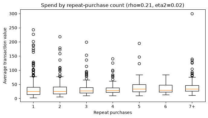
Spearman rho comes out 0.21 across 1,139 repeat buyers, and the spread inside each box dwarfs the drift between boxes. The assumption holds on CDNOW. It won’t hold everywhere, which is why the check runs by default rather than living in a doc.
Plot and export#
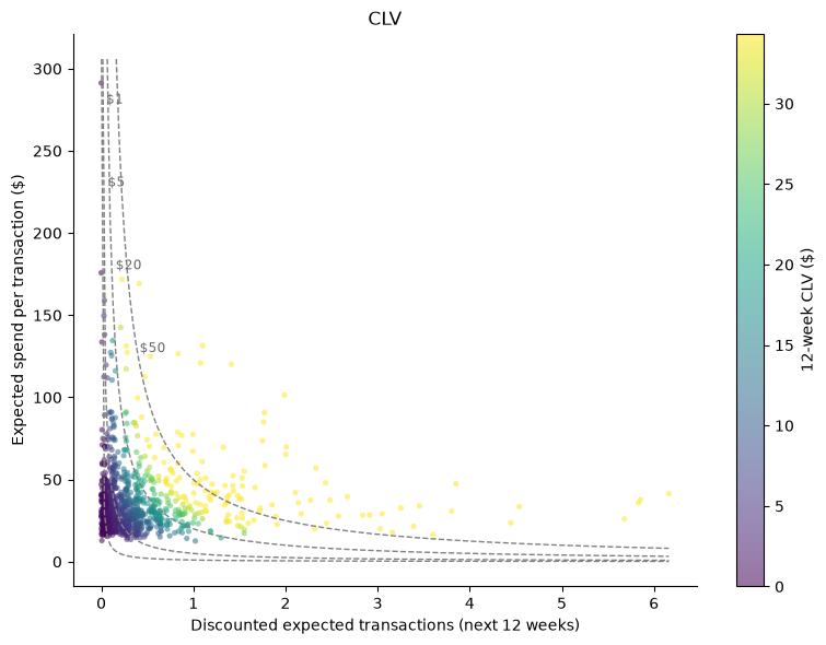
Every clvkit result draws itself and hands back a plain DataFrame. to_pandas() is the escape hatch, so nothing here is a trap.
[22]:
fig, ax = plt.subplots(figsize=(8, 6))
result.plot(
    ax=ax,
    scatter_kwargs={"s": 14, "alpha": 0.55, "edgecolors": "none"},
    title="CLV",
)
# ax.set_xlim(0, 20)
# ax.set_ylim(0, 60)
fig.tight_layout()
[19]:
csv_path = OUTPUT / "cdnow_clv.csv"
result.to_pandas().to_csv(csv_path)
print(f"wrote {csv_path.relative_to(REPO)} ({csv_path.stat().st_size:,} bytes)")

result.to_pandas().nlargest(5, "clv").round(2)
wrote examples/output/cdnow_clv.csv (192,544 bytes)
[19]:
| expected_purchases | discounted_expected_transactions | expected_spend | clv | |
|---|---|---|---|---|
| customer_id | ||||
| 1981 | 6.20 | 6.16 | 41.44 | 255.37 |
| 1203 | 5.89 | 5.86 | 37.71 | 220.77 |
| 1516 | 5.87 | 5.83 | 35.81 | 208.88 |
| 1081 | 2.00 | 1.99 | 101.32 | 201.56 |
| 2149 | 3.88 | 3.85 | 47.43 | 182.70 |
8. What time_unit="W" does on its own#
time_unit="W" without collapse doesn’t merely re-scale the ruler. It buckets events at weekly grain, merging a Monday and a Wednesday purchase into one. That’s a coarser sufficient statistic than the published fit used, and it takes the most from the most frequent buyers, whose behaviour is the whole reason to fit a model.
CustomerBase won’t do it silently. Naming the grain is consent to it. Inheriting it is the trap.
[20]:
import warnings

with warnings.catch_warnings(record=True) as caught:
    warnings.simplefilter("always")
    coarse = CustomerBase.from_transactions(log, amount_col=None, time_unit="W")
    for warning in caught:
        print(f"{warning.category.__name__}: {warning.message}\n")

coarse_cal, _ = coarse.split(calibration_period_end="1997-09-30")
coarse_params = BGNBD().fit(coarse_cal).params_

pd.DataFrame(
    {
        "published": published,
        'collapse="D"': model.params_,
        "collapsed weekly": coarse_params,
    }
).round(3)
UserWarning: time_unit='W' collapsed 558 of 6919 transactions into earlier purchases in the same period. This biases the fit downward, and it takes the most from your most frequent buyers. Pass collapse='D' to keep them and still report time in 'W', or pass collapse='W' to say you meant this.
[20]:
| published | collapse="D" | collapsed weekly | |
|---|---|---|---|
| r | 0.243 | 0.243 | 0.291 |
| alpha | 4.414 | 4.414 | 6.852 |
| a | 0.793 | 0.793 | 0.665 |
| b | 2.426 | 2.426 | 2.320 |
Alpha moves 55%, from 4.41 to 6.85. Nothing raised, and the optimiser converged happily onto the wrong sufficient statistic. A fit that fails loudly is cheap to debug; this one doesn’t, so the warning has to carry the whole signal.
9. Exercise#
CLV accepts any transaction model with fit and predict(t). The coupling is structural, not an inheritance hierarchy. MBG/NBD is the never-returner variant of BG/NBD, and it lets a customer drop out immediately after a purchase, which BG/NBD forbids.
Refit lifetime value with MBGNBD() as the transaction model and compare its clv column against the BG/NBD one. Which direction does the mean move, and would you expect that from a model that lets customers leave sooner? Run the cell below for one answer, then try horizon=104 to see whether the gap widens.
[21]:
from clvkit import MBGNBD

mbg_result = (
    CLV(transaction_model=MBGNBD()).fit(cb).predict(horizon=52, discount_rate=0.001)
)

side_by_side = pd.DataFrame(
    {
        "clv_bgnbd": result.to_pandas()["clv"],
        "clv_mbgnbd": mbg_result.to_pandas()["clv"],
    }
)
side_by_side["delta"] = side_by_side["clv_mbgnbd"] - side_by_side["clv_bgnbd"]
side_by_side.describe().round(2)
[21]:
| clv_bgnbd | clv_mbgnbd | delta | |
|---|---|---|---|
| count | 2349.00 | 2349.00 | 2349.00 |
| mean | 7.73 | 29.48 | 21.75 |
| std | 18.92 | 72.62 | 53.72 |
| min | 0.00 | 0.00 | 0.00 |
| 25% | 1.36 | 3.94 | 2.57 |
| 50% | 1.45 | 4.29 | 2.84 |
| 75% | 5.36 | 21.93 | 16.71 |
| max | 255.37 | 949.17 | 693.80 |
Where to go next#
opinions.md in the repo root separates canon, what the papers settle, from opinion, what clvkit chose, for every default you just accepted. docs/references.md has the DOIs. None of the papers carries a redistribution licence, so fetch them from there. examples/online_retail_ii_cohort.ipynb covers the descriptive half of the library, where there is no likelihood at all.