Online Retail II: cohort retention and revenue

Audience. An analyst who wants the descriptive half of clvkit, which reports what the transaction log already says before any model is fit.

Prerequisites. uv sync, plus network access on the first run. This notebook downloads the UCI Online Retail II dataset, 43 MB, and caches it under examples/data/. Later runs are offline.

Data. UCI Machine Learning Repository — Online Retail II, licensed CC BY 4.0. CDNOW, used by the other examples, ships in the repository; this is the one dataset not vendored, so grab it from that page if you’d rather not let the notebook fetch it. Section 1 downloads and caches it automatically.

Learning goals. By the end you can:

1. Say what a cohort is, and build a cohort matrix by hand on six customers.

2. Clean a real retail log into the (customer_id, date, amount) contract every clvkit entry point consumes.

3. Build a CohortMatrix of retention and one of revenue, and read the triangle.

4. Say why an unobserved cell is NaN and never 0, and why that distinction is the reason the chart can be trusted.

Nothing below assumes you’ve built a cohort matrix before. Section 0 builds one from six invented customers you can check by counting, and only then does the real dataset arrive.

If you’re coming from examples/cdnow_clv.ipynb, none of the BTYD vocabulary carries over. There’s no model here, no likelihood, and no recency.

Outline

0. What a cohort matrix is, on six customers

1. Fetch and cache the dataset

2. Line items to the transaction-log contract

3. Retention, and the triangle

4. Revenue, the same pivot with a different cell

5. Relative against absolute, and getting the data out

6. Exercise

0. What a cohort matrix is, on six customers

The idea

“Retention was 34% last month” is a number that can’t be acted on, because it mixes customers who arrived two years ago with customers who arrived in March. A cohort unmixes them: everyone who made their first purchase in the same period is grouped together and followed forward on their own clock.

That gives a table with a specific shape:

• one row per acquisition cohort, labelled by the period of first purchase

• one column per ``period_number``, meaning whole periods elapsed since that cohort’s own start, so column 0 is always the cohort’s own period

• one number per cell, either how many of them were active or how much they spent

Because each row runs on its own clock, the same column means “one month in” for every cohort, whether that cohort started in 2009 or in 2011. That’s the whole trick, and it’s why the columns are comparable down a page.

The glossary

Term	What it means here	Watch out
Acquisition cohort	Every customer whose first observed purchase falls in the same period.	Assigned once, from the log. A customer never changes cohort.
``period_number``	Whole periods elapsed since the cohort’s own period.	Column 0 is the cohort’s own period, so relative column 0 is always 1.0.
Retention cell	Distinct customers of that cohort active in that period.	A customer buying three times in one month counts once.
Revenue cell	Total spend by that cohort in that period.	A sum, so one big order moves it. Retention wouldn’t budge.
Relative view	Each row divided by its own column 0.	The comparable view, since cohorts differ in size.
Absolute view	Raw counts or raw currency.	Answers “how many” and “how much”, not “how fast do they decay”.
The triangle	Older cohorts have more observed columns, so the filled area is a triangle.	The empty corner is NaN, not 0. That distinction is section 3.

There’s no fit() anywhere in this notebook. Every cell is a count or a sum of things that already happened, so nothing here needs a model to be believed.

Build one by hand

Six customers, four months, small enough to check by counting.

import matplotlib.pyplot as plt
import pandas as pd

from clvkit import CohortMatrix

# Same role-based colours as the CDNOW notebook, validated as a set for
# colour-vision deficiency. Here they identify cohorts rather than spans.
SURFACE, INK, MUTED, GREY = "#fcfcfb", "#0b0b0b", "#52514e", "#d8d7d2"
COHORT_COLOURS = ["#2a78d6", "#eb6834", "#1baf7a"]

toy = pd.DataFrame(
    [
        ("C1", "2024-01"),
        ("C1", "2024-02"),
        ("C1", "2024-04"),
        ("C2", "2024-01"),
        ("C3", "2024-01"),
        ("C3", "2024-03"),
        ("C4", "2024-02"),
        ("C4", "2024-03"),
        ("C5", "2024-02"),
        ("C6", "2024-04"),
    ],
    columns=["customer_id", "month"],
).assign(date=lambda d: pd.to_datetime(d["month"]), amount=10.0)

toy_matrix = CohortMatrix.from_transactions(toy, period="M", metric="retention")
toy_matrix.to_pandas()

period_number	0	1	2	3
cohort
2024-01	3.0	1.0	1.0	1.0
2024-02	2.0	1.0	0.0	NaN
2024-04	1.0	NaN	NaN	NaN

Check a few cells against the list above before reading on.

Row 2024-01 holds C1, C2 and C3, so column 0 is 3. Column 1 is January’s customers active in February, which is C1 alone, so 1. Column 3 is January’s customers active in April, which is C1 again.

Row 2024-02 holds C4 and C5. Column 2 is February’s customers active in April, and neither of them bought in April, so that cell is 0. They were watched and they didn’t come.

Row 2024-04 holds C6 alone. Columns 1 to 3 would be May, June and July, which haven’t happened. Those cells are NaN, and they mean something completely different from the zero above them.

The next cell draws both halves: the log on the left, the matrix it produces on the right.

periods = pd.period_range("2024-01", "2024-04", freq="M")
toy_period = toy["date"].dt.to_period("M")
cohort_of = toy_period.groupby(toy["customer_id"]).min()
customers = sorted(toy["customer_id"].unique(), key=lambda c: (cohort_of[c], c))
colour_of = {p: COHORT_COLOURS[i] for i, p in enumerate(sorted(cohort_of.unique()))}

fig, (left, right) = plt.subplots(1, 2, figsize=(12.5, 4.2), width_ratios=[1, 1.15])
fig.patch.set_facecolor(SURFACE)

# ---- left: the raw log -------------------------------------------------------
left.set_facecolor(SURFACE)
for row, cid in enumerate(customers):
    y = len(customers) - row - 1
    colour = colour_of[cohort_of[cid]]
    bought = toy_period[toy["customer_id"] == cid]
    left.plot([0, len(periods) - 1], [y, y], color=GREY, lw=1, zorder=1)
    for p in bought:
        x = (p - periods[0]).n
        first = p == cohort_of[cid]
        left.scatter(
            x,
            y,
            s=190 if first else 110,
            color=colour,
            zorder=3,
            edgecolor=INK if first else SURFACE,
            linewidth=1.4,
        )
    left.text(-0.55, y, cid, va="center", ha="right", fontsize=10, color=INK)

left.set_xticks(range(len(periods)), [str(p) for p in periods], fontsize=9)
left.set_yticks([])
left.set_xlim(-1.35, len(periods) - 0.6)
left.set_ylim(-0.9, len(customers) - 0.4)
left.set_title("The log: who bought when", loc="left", fontsize=11)
left.text(
    -1.3,
    -0.62,
    "ringed dot = first purchase, which fixes the cohort",
    fontsize=8.5,
    color=MUTED,
)
for side in ("top", "right", "left", "bottom"):
    left.spines[side].set_visible(False)
left.tick_params(colors=MUTED, length=0)

# ---- right: the matrix it produces -------------------------------------------
right.set_facecolor(SURFACE)
grid = toy_matrix.to_pandas()
for row, (cohort, values) in enumerate(grid.iterrows()):
    y = len(grid) - row - 1
    for col, value in enumerate(values):
        observed = pd.notna(value)
        right.add_patch(
            plt.Rectangle(
                (col - 0.44, y - 0.36),
                0.88,
                0.72,
                facecolor=colour_of[cohort] if observed else "#ececea",
                alpha=0.9 if observed else 1.0,
                edgecolor=SURFACE,
                linewidth=2,
            )
        )
        right.text(
            col,
            y,
            f"{value:.0f}" if observed else "NaN",
            ha="center",
            va="center",
            fontsize=11,
            color="white" if observed else MUTED,
            fontweight="bold" if observed else "normal",
        )
    right.text(-0.75, y, str(cohort), va="center", ha="right", fontsize=10, color=INK)

right.set_xticks(range(grid.shape[1]), [str(c) for c in grid.columns], fontsize=9)
right.set_yticks([])
right.set_xlim(-1.9, grid.shape[1] - 0.4)
right.set_ylim(-0.9, len(grid) - 0.4)
right.set_xlabel("period_number: months since that cohort's own month", color=MUTED)
right.set_title("The matrix: active customers per cohort", loc="left", fontsize=11)
right.text(
    -1.85, -0.62, "grey NaN = hasn't happened yet, not zero", fontsize=8.5, color=MUTED
)
for side in ("top", "right", "left", "bottom"):
    right.spines[side].set_visible(False)
right.tick_params(colors=MUTED, length=0)

fig.tight_layout()

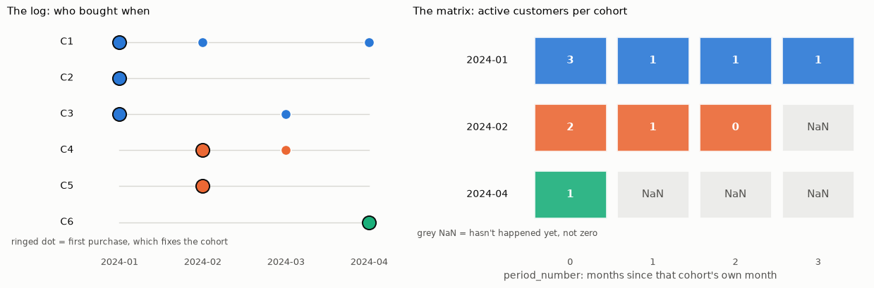
The left panel is the log. The right panel is the same information counted differently, and every number on the right can be traced back to dots on the left.

Two cells are worth staring at, because they look alike and aren’t.

The 2024-02 row ends with a solid 0 at period_number = 2. April happened, February’s cohort was there to be counted, and nobody bought. That’s a fact about the customers.

The 2024-04 row is grey from period_number = 1 onwards. May hasn’t happened. That’s a fact about the window, not about the customers, and filling it with 0 would invent a churn event out of a calendar. This is why CohortMatrix returns a triangle, and why the retention matrix is float-typed even though it counts whole customers: those NaNs have to live somewhere.

Now the same operation on 5,878 real customers.

1. Fetch and cache the dataset

Online Retail II is a UK gift-ware retailer’s transaction log from December 2009 to December 2011: 1,067,371 line items and 5,878 identified customers. CDNOW is a single 1997 acquisition cohort, so it can’t demonstrate a cohort matrix at all. Here customers keep arriving across the two years, which yields 25 natural monthly acquisition cohorts.

It’s CC BY 4.0 and redistributable, but it is fetched rather than vendored. 43 MB in every clone forever costs more than the offline build is worth. The cost of that choice: a UCI outage turns this notebook red in CI, and that is the only part of the build depending on a third party being up.

Source: https://archive.ics.uci.edu/dataset/502/online+retail+ii. Cited in docs/references.md under Data.

import urllib.request
import zipfile
from pathlib import Path

URL = "https://archive.ics.uci.edu/static/public/502/online+retail+ii.zip"

# Anchored to the repo, not to Path.cwd(), so the 43 MB download and the exported
# artifacts land where .gitignore covers them however the kernel was started.
REPO = next(
    p for p in [Path.cwd(), *Path.cwd().parents] if (p / "CDNOW_sample.txt").exists()
)
DATA = REPO / "examples" / "data"
OUTPUT = REPO / "examples" / "output"
DATA.mkdir(parents=True, exist_ok=True)
OUTPUT.mkdir(parents=True, exist_ok=True)

archive = DATA / "online_retail_ii.zip"
workbook = DATA / "online_retail_II.xlsx"

if not workbook.exists():
    if not archive.exists():
        print(f"downloading {URL} ...")
        urllib.request.urlretrieve(URL, archive)
    with zipfile.ZipFile(archive) as zf:
        zf.extract("online_retail_II.xlsx", DATA)

print(f"{workbook.relative_to(REPO)} ({workbook.stat().st_size / 1e6:.0f} MB)")

examples/data/online_retail_II.xlsx (46 MB)

The workbook holds one sheet per year. Reading both takes about 20 seconds, and there’s no faster path that keeps the source honest.

sheets = pd.read_excel(workbook, sheet_name=None)
lines = pd.concat(sheets.values(), ignore_index=True)

print({name: len(df) for name, df in sheets.items()})
lines.head()

{'Year 2009-2010': 525461, 'Year 2010-2011': 541910}

	Invoice	StockCode	Description	Quantity	InvoiceDate	Price	Customer ID	Country
0	489434	85048	15CM CHRISTMAS GLASS BALL 20 LIGHTS	12	2009-12-01 07:45:00	6.95	13085.0	United Kingdom
1	489434	79323P	PINK CHERRY LIGHTS	12	2009-12-01 07:45:00	6.75	13085.0	United Kingdom
2	489434	79323W	WHITE CHERRY LIGHTS	12	2009-12-01 07:45:00	6.75	13085.0	United Kingdom
3	489434	22041	RECORD FRAME 7" SINGLE SIZE	48	2009-12-01 07:45:00	2.10	13085.0	United Kingdom
4	489434	21232	STRAWBERRY CERAMIC TRINKET BOX	24	2009-12-01 07:45:00	1.25	13085.0	United Kingdom

2. Line items to the transaction-log contract

The real-world warts, and what each one does to a cohort matrix if it survives:

Wart	Rows dropped	Why it goes
Missing Customer ID	243,007 (22.8%)	No customer, no cohort. These are unidentified walk-up sales.
Cancellations, Invoice starting C	18,744 (1.8%)	Negative quantities. A refund isn’t a purchase event.
Non-positive Quantity or Price	71 (0.01%)	Adjustments and write-offs, not trade.

Then line items aggregate to invoices, because one basket is one purchase event. clvkit reads a log of purchase events rather than of SKUs, and the difference has teeth. A 40-line Christmas order is one act of buying, not forty, and feeding the line items straight in would tell every model that this customer shops 40 times a day.

clean = lines.dropna(subset=["Customer ID"])
clean = clean[~clean["Invoice"].astype(str).str.startswith("C")]
clean = clean[(clean["Quantity"] > 0) & (clean["Price"] > 0)]
clean = clean.assign(
    customer_id=clean["Customer ID"].astype("int64"),
    line_amount=clean["Quantity"] * clean["Price"],
)

orders = clean.groupby(["customer_id", "Invoice"], as_index=False).agg(
    date=("InvoiceDate", "min"),
    amount=("line_amount", "sum"),
)

print(f"{len(lines):,} line items -> {len(clean):,} kept -> {len(orders):,} orders")
print(
    f"{orders['customer_id'].nunique():,} customers, "
    f"{orders['date'].min():%Y-%m-%d} to {orders['date'].max():%Y-%m-%d}"
)
orders.head()

1,067,371 line items -> 805,549 kept -> 36,969 orders
5,878 customers, 2009-12-01 to 2011-12-09

	customer_id	Invoice	date	amount
0	12346	491725	2009-12-14 08:34:00	45.0
1	12346	491742	2009-12-14 11:00:00	22.5
2	12346	491744	2009-12-14 11:02:00	22.5
3	12346	492718	2009-12-18 10:47:00	22.5
4	12346	492722	2009-12-18 10:55:00	1.0

805,549 of 1,067,371 line items survive, and they collapse into 36,969 orders. That’s 137 line items per customer against 6.3 purchases per customer. Feed the line items in and every model here is told this base shops 20 times more often than it does.

3. Retention, and the triangle

CohortMatrix is the one part of clvkit with no likelihood, no fitting and no parameters. Every cell is an observed count or an observed sum, so nothing here needs the BTYD canon to be believed. There is no fit(), because a pivot has no state to estimate.

It reads the raw log rather than a CustomerBase. An RFM summary keeps only first and last purchase timing, and a cohort matrix needs the whole per-period activity pattern. A customer who bought in months 0, 3 and 7 is indistinguishable in RFM from one who bought in 0, 5 and 7.

retention = CohortMatrix.from_transactions(orders, period="M", metric="retention")
print(repr(retention))

retention.to_pandas(relative=True).iloc[:6, :8].round(3)

<CohortMatrix 'retention' 25 cohorts x 25 'M' periods>

period_number	0	1	2	3	4	5	6	7
cohort
2009-12	1.0	0.353	0.334	0.425	0.380	0.359	0.377	0.342
2010-01	1.0	0.206	0.311	0.305	0.264	0.300	0.258	0.230
2010-02	1.0	0.238	0.225	0.291	0.246	0.201	0.193	0.286
2010-03	1.0	0.190	0.230	0.242	0.233	0.203	0.246	0.302
2010-04	1.0	0.194	0.194	0.163	0.184	0.224	0.276	0.262
2010-05	1.0	0.157	0.169	0.173	0.177	0.256	0.213	0.126

Rows are acquisition cohorts, the month of a customer’s first observed purchase. Columns are whole months elapsed since that cohort’s own month. Column 0 is the cohort itself, so relative column 0 is 1.0 by construction.

The triangle is what makes the chart honest. Recent cohorts have been observed for fewer months, so cells past a cohort’s observation window are NaN, never 0. A zero means observed and nobody bought. Missing means not yet knowable. Conflating the two is how a young cohort gets read as a cohort that churned. The cost, stated in the class docstring: the retention matrix is float-typed even though it counts customers, because those NaNs have to live somewhere.

absolute = retention.to_pandas()
last_cohort = absolute.index[-1]

print(f"newest cohort: {last_cohort}")
print(f"observed cells in that row: {int(absolute.loc[last_cohort].notna().sum())}")
print(f"unobserved (NaN) cells:     {int(absolute.loc[last_cohort].isna().sum())}")
print(f"\nobserved zeros anywhere in the matrix: {int((absolute == 0).sum().sum())}")

newest cohort: 2011-12
observed cells in that row: 1
unobserved (NaN) cells:     24

observed zeros anywhere in the matrix: 0

fig, ax = plt.subplots(figsize=(16, 9))
retention.plot(ax=ax, relative=True)
ax.set_title("Online Retail II, monthly retention rate")
fig.tight_layout()
fig.savefig(OUTPUT / "online_retail_ii_retention.png", dpi=110)

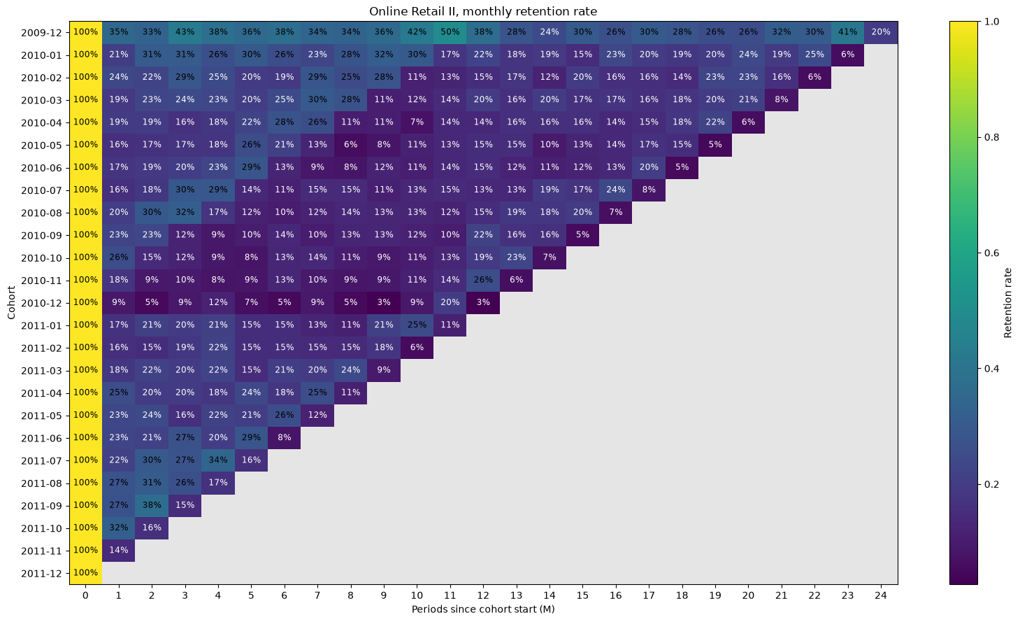
Unobserved cells are drawn in flat grey and left unlabelled, so the eye never reads them as a cohort that dropped to zero.

The 2009-12 row is the one to read across. It’s the only cohort observed for the full two years, and it holds 33% to 50% of its customers month after month, while the twelve cohorts acquired during 2010 average 17% to 20% over their first six months. Roughly double, and it holds for two solid years.

That gap is the surprising number here, and the flattering reading is not the likely one. December 2009 is the first month in the file, so anyone already loyal to this retailer before the data starts gets labelled a 2009-12 acquisition. The cohort is contaminated by survivors on the left edge of the window. Every cohort matrix built on a log that doesn’t reach back to the company’s founding has this problem in its top row.

The narrower rows below are not worse cohorts. They’re younger ones.

4. Revenue, the same pivot with a different cell

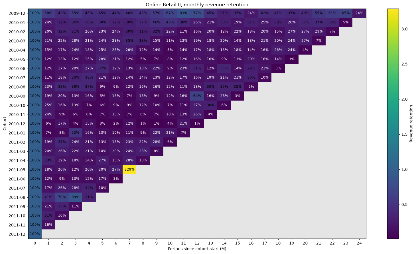
metric="revenue" sums amounts instead of counting distinct customers. Relative mode then divides each cohort by its own month-0 revenue, giving a revenue index: how much of its opening month’s spend a cohort still generates.

This is the number that pays for things, and it routinely diverges from headcount retention. A cohort can lose most of its customers and keep most of its revenue.

revenue = CohortMatrix.from_transactions(orders, period="M", metric="revenue")
print(repr(revenue))

fig, ax = plt.subplots(figsize=(16, 9))
revenue.plot(ax=ax, relative=True)
ax.set_title("Online Retail II, monthly revenue retention")
fig.tight_layout()
fig.savefig(OUTPUT / "online_retail_ii_revenue.png", dpi=110)

<CohortMatrix 'revenue' 25 cohorts x 25 'M' periods>

oldest = retention.to_pandas().index[0]
side_by_side = pd.DataFrame(
    {
        "customer_retention": retention.to_pandas(relative=True).loc[oldest],
        "revenue_retention": revenue.to_pandas(relative=True).loc[oldest],
    }
).dropna()

side_by_side.head(13).round(3)

	customer_retention	revenue_retention
period_number
0	1.000	1.000
1	0.353	0.576
2	0.334	0.432
3	0.425	0.553
4	0.380	0.447
5	0.359	0.446
6	0.377	0.441
7	0.342	0.457
8	0.336	0.484
9	0.362	0.572
10	0.422	0.672
11	0.495	0.835
12	0.376	0.771

Revenue retention beats customer retention in 23 of the 2009-12 cohort’s 25 months. At month 11 it’s 49.5% of the customers producing 83.5% of the opening month’s revenue. The ones who stayed are the ones who spend, so reporting only the left-hand column understates what the cohort is worth by a factor that grows over its life.

5. Relative against absolute, and getting the data out

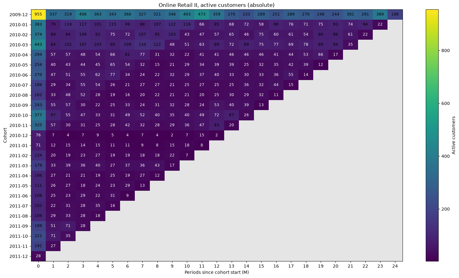
plot() defaults to relative=True, because that’s what the chart is read for: how fast each cohort decays, independent of how big it was. The absolute view answers a different question, which is how many customers and how much money.

fig, ax = plt.subplots(figsize=(16, 9))
retention.plot(ax=ax, relative=False)
ax.set_title("Online Retail II, active customers (absolute)")
fig.tight_layout()

retention.to_pandas(relative=True).to_csv(OUTPUT / "online_retail_ii_retention.csv")
revenue.to_pandas(relative=True).to_csv(OUTPUT / "online_retail_ii_revenue.csv")

# to_json keeps the triangle legible outside pandas: unobserved cells are null.
print(revenue.to_json(relative=True)[:220], "...")
print("\nwrote:", *sorted(p.name for p in OUTPUT.iterdir()), sep="\n  ")

{"2009-12":{"0":1.0,"1":0.5758729708,"2":0.4322439873,"3":0.5529049587,"4":0.4469292373,"5":0.4455720329,"6":0.4410627324,"7":0.4565656895,"8":0.4842304312,"9":0.5718104438,"10":0.672265992,"11":0.8346691761,"12":0.77144 ...

wrote:
  cdnow_clv.csv
  online_retail_ii_retention.csv
  online_retail_ii_retention.png
  online_retail_ii_revenue.csv
  online_retail_ii_revenue.png

6. Exercise

period is any pandas offset alias, and it sets both the cohort grain and the column grain, because a cohort matrix only makes sense when both use the same clock.

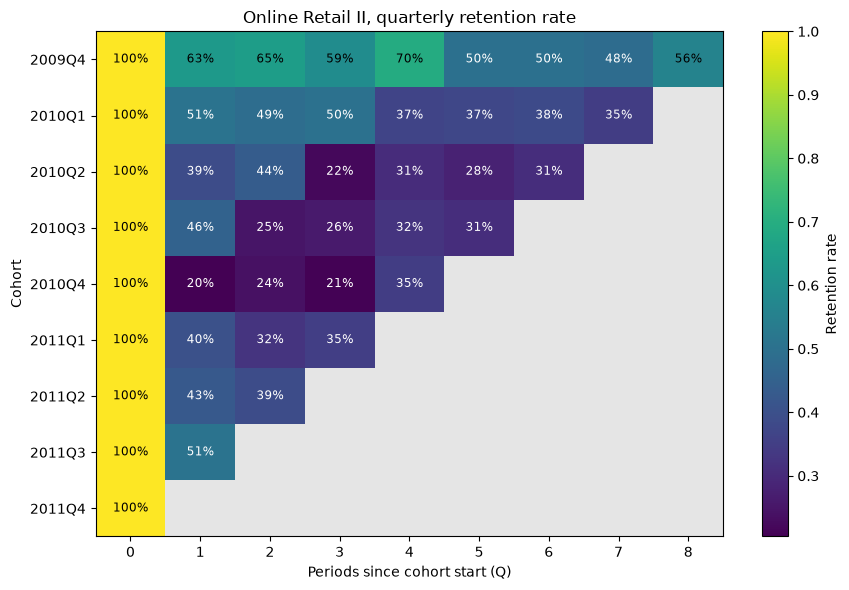
Rebuild the retention matrix at period="Q". Quarterly cohorts are larger and less noisy, but you lose the within-quarter decay the monthly view shows. Which of the two would you put in front of a finance team, and which in front of lifecycle marketing? Run the cell below, then try period="W" to watch the triangle become unreadable.

quarterly = CohortMatrix.from_transactions(orders, period="Q", metric="retention")
print(repr(quarterly))

fig, ax = plt.subplots(figsize=(9, 6))
quarterly.plot(ax=ax, relative=True)
ax.set_title("Online Retail II, quarterly retention rate")
fig.tight_layout()

quarterly.to_pandas(relative=True).round(3)

<CohortMatrix 'retention' 9 cohorts x 9 'Q' periods>

period_number	0	1	2	3	4	5	6	7	8
cohort
2009Q4	1.0	0.631	0.648	0.591	0.695	0.497	0.498	0.485	0.56
2010Q1	1.0	0.508	0.488	0.502	0.367	0.374	0.382	0.349	NaN
2010Q2	1.0	0.390	0.435	0.220	0.306	0.281	0.308	NaN	NaN
2010Q3	1.0	0.455	0.250	0.261	0.323	0.310	NaN	NaN	NaN
2010Q4	1.0	0.204	0.240	0.208	0.348	NaN	NaN	NaN	NaN
2011Q1	1.0	0.401	0.324	0.353	NaN	NaN	NaN	NaN	NaN
2011Q2	1.0	0.428	0.391	NaN	NaN	NaN	NaN	NaN	NaN
2011Q3	1.0	0.506	NaN	NaN	NaN	NaN	NaN	NaN	NaN
2011Q4	1.0	NaN	NaN	NaN	NaN	NaN	NaN	NaN	NaN

Where to go next

CohortSurvival answers a similar question with a model behind it: aggregated BG/NBD P(alive) per cohort, which extrapolates past the observation window capping this matrix. It also carries a cost worth knowing, since a survival curve is a cross-section across cohorts and not a panel followed forward. examples/cdnow_clv.ipynb covers the modelled half, reproducing the published Fader-Hardie estimates and composing them into lifetime value.